Apache Cassandra and the Cassandra Query Language (CQL) have evolved over the past couple of years. Key improvements include:
- Significant storage engine improvements
- Introduction of SSTable Attached Secondary Index i.e SASI Indexes
- Materialized views
- Simple role based authentication
This post is an updated to “A Practical Introduction to Cassandra Query Language”. The tutorial will concentrate on two things:
- Cassandra Query Language and its interaction with the new storage engine.
- Introducing the various CQL statements via a practical example.
CQL Overview
Cassandra Query Language or CQL is a data management language akin to SQL. CQL is a simple API over Cassandra’s internal storage structures. Apache Cassandra introduced CQL in version 0.8. Thrift an RPC-based API was the preferred data management language prior to the introduction of CQL. CQL provides a flatter learning curve in comparison to Thrift and thus its is the preferred way of interacting with Apache Cassandra. In fact, Thrift support is slated to be removed in Apache Cassandra 4.0 release.
CQL has many restrictions in comparison to SQL. These restrictions prevent inefficient querying across a distributed database. CQL queries should not visit a large number of nodes to retrieve required data. This has the potential to impact cluster-wide performance. Thus CQL prevents the following:
- No arbitrary WHERE clause – Apache Cassandra prevents arbitrary predicates in a WHERE statement. Where clauses must have columns specified in your primary key.
- No JOINS – You cannot join data from two Apache Cassandra tables.
- No arbitrary GROUP BY – GROUP BY can only be applied to a partition or cluster column. Apache Cassandra 3.10 added GROUP BY support to SELECT statements.
- No arbitrary ORDER BY clauses – Order by can only be applied to a clustered column.
CQL Fundamentals
Let’s start off by understanding some basic concepts i.e. cluster, keyspaces, tables aka column family and primary key.
- Apache Cassandra Cluster – A cluster is a group of computers working together that are viewed as a single system. A distributed database is a database system that is spread across a cluster. Apache Cassandra is a distributed database spread across a cluster of nodes. Think of Apache Cassandra Cluster as a database server spread across a number of machines.
- Keyspaces – A keyspace is similar to an RDBMS schema/database. A keyspace is a logical grouping of Apache Cassandra tables. Like a database, a keyspace has attributes that define system-wide behaviour. Two key attributes are the replication factor and the replication strategy. The replication factor defines the number of replicas the replication strategy defines the algorithm used to determine the placement of the replicas.
- Tables – An Apache Cassandra table is similar to an RDBMS table. Like in an RDBMS a table is made up of a number of rows. This is where the similarity ends. Think of an Apache Cassandra table as a map of sorted maps. A table contains rows each of which is accessible by the partition key. The row contains column data which are ordered by the clustering key. Visualise an Apache Cassandra table as a map of sorted maps spread across a cluster of nodes.
- Primary Key – A Primary key uniquely identifies an Apache Cassandra row. A primary key can be a simple key or a composite key. A composite key is made up of two parts, a partition key and a cluster key. The partition key determines data distribution in the cluster while the cluster key determines sort order within a partition.
The diagram below helps visualise the above concepts.
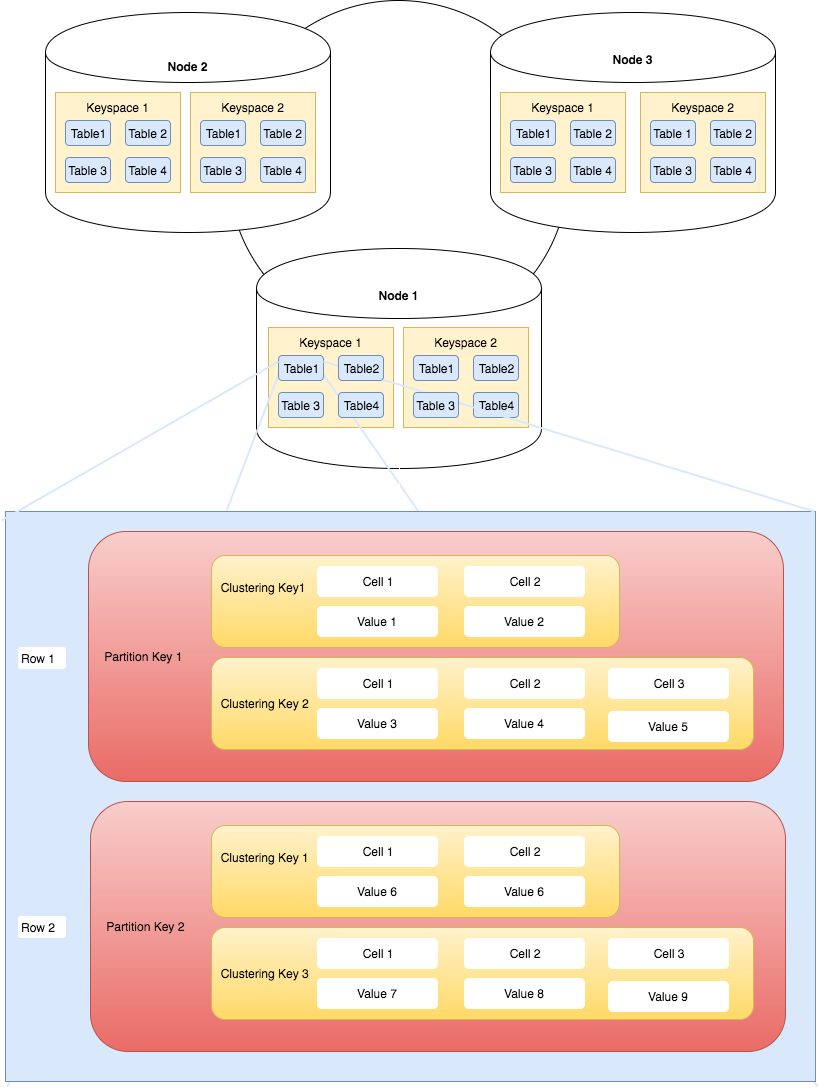
Apache Cassandra Cluster, Keyspace, Table and Primary Key Overview
Notice how keyspaces and tables are spread across the cluster. In summary, Apache Cassandra cluster contains keyspaces. Keyspaces contain tables. Tables contain rows which are retrieved via their primary key. The goal is to distribute this data across a cluster of nodes.
Installing Cassandra
To go through this tutorial you need Apache Cassandra installed. You can either use a Docker base Apache Cassandra installation or use any of the installation methods laid out in 5 ways to install Apache Cassandra. I will be using the Docker base Cassandra installation.
CQLSH
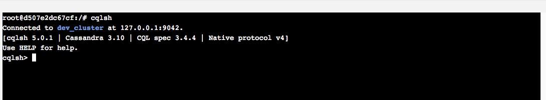
Cqlsh is a Python based utility that enables you to execute CQL. A cqlsh prompt can be obtained by simply executing the cqlsh utility. In the Docker-based installation navigate to the containers command prompt. Once at the command prompt simply type cqlsh. For native installs the cqlsh utility can be found in CASSANDRA_INSTALLTATION_DIR/bin. Executing the cqlsh utility will take you to the cqlsh prompt.
CQL By Examples
Navigating an Apache Cassandra Cluster
The first things you need to get familiar with is navigating around a cluster. The DESCRIBE command, or DESC or shorthand, is the key to navigating around the cluster. The DESCRIBE command can be used to list cluster objects such as keyspaces, tables, types, functions, aggregates. It can also be used to output CQL commands to recreate a keyspace, table, index, materialized view, schema, function, aggregate or any CQL object. To get a full list of DESCRIBE command options please type HELP DESC at the cqlsh prompt. The HELP provided is self-explanatory.
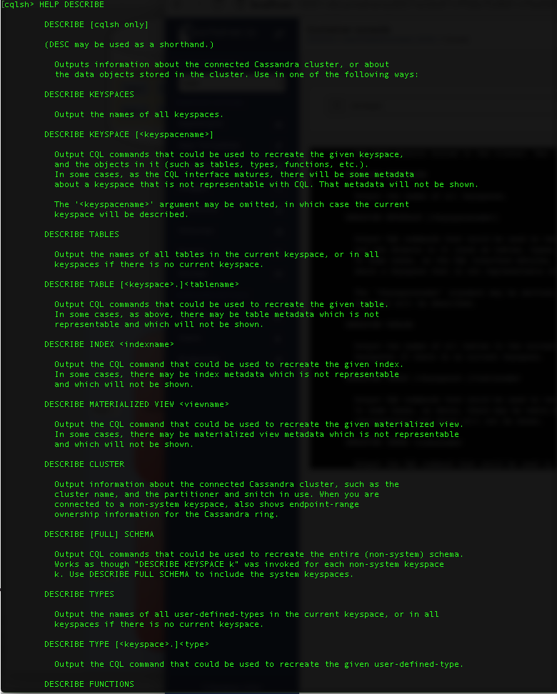
Describe command help
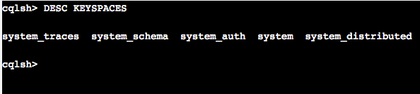
Often the first thing you want to do when you are the CQLSH prompt is to list keyspaces. The
|
1 |
DESCRIBE KEYSPACES |
command provides a list of all keyspace. Go ahead and execute this command. Since we have freshly installed Apache Cassandra all you will see a list of system keyspaces. Systems keyspaces help Apache Cassandra to keep track of cluster and node related metadata.
Here are a couple of gotchas. There is no command to list all indexes. To list indexes you have to query the system keyspace. To list all indexed you will need to execute the following command:
|
1 |
SELECT * FROM system.”IndexInfo”; |
Similarly, there is no command to list all materialized views. To get a list of all the views you must execute the following command:
|
1 |
SELECT * FROM system_schema.views; |
CQL Create Keyspace
Let’s create our first keyspace. The keyspace is called animals. Execute the statement below to create the animal keyspace.
|
1 |
CREATE KEYSPACE animals WITH REPLICATION = { 'class' : 'SimpleStrategy' , 'replication_factor' : 3 }; |
Two key parameters to take note of is the class and the replication factor. The class defines the replication strategy i.e. algorithm used to determine the placement of the replicas. The replication factor determines the number of replicas. Since I have three node cluster I have chosen a replication factor of 3.
Execute the
|
1 |
DESC KEYSPACES |
command once more to see if the aminal keyspace is created. Next, let’s connect to the created keyspace with the help the of the USE command. The USE command enables switching context between keyspaces. Once a keyspace is chosen all subsequent commands are executed in the context of the chosen keyspace. Please execute
|
1 |
USE animals; |
CQL Create Table
Let’s create a table called monkeys in the animals keyspace. Execute the following command to create the monkey table.
|
1 2 3 4 5 6 7 8 |
CREATE TABLE monkeys ( type text, family text, common_name text, conservation_status text, avg_size_in_grams int, PRIMARY KEY ((type, family), common_name) ); |
Take special note of the primary key. The primary key defined above is a composite key. The primary key has two parts. i.e. partition key and cluster key. The first column of the primary key is your partition key. The remaining columns are used to determine the cluster key. A composite partition key, a partition key made up of multiple columns, is defined by using an extra set of parentheses before the clustering columns. The partition key helps distribute data across the cluster while the cluster key determines the order of the data stored within a row. Thus type and family is our composite partition key and common_name is our cluster key. When designing a table think of the partition key as a tool to spread data evenly across a cluster while the cluster key helps determine the order of that data within a partition. Your data and query patterns will influence your primary key. Please note the cluster key is optional.
CQL INSERT
Let’s insert some data into above table. When inserting data the primary key is mandatory.
|
1 2 |
INSERT INTO monkeys (type, family, common_name, conservation_status) VALUES ('New World Monkey', 'Cebidae', 'white-headed capuchin', 'Least concern'); |
Execute a select statement to see that the data has been inserted successfully.
|
1 |
SELECT * FROM monkeys; |
You should see the following output:
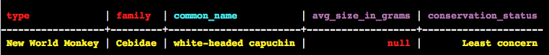
Note columns in red are your partition key. Cyan coloured columns are your cluster key. The columns in purple are the rest of your columns.
CQL Consistency Level
Cassandra enables users to configure the number of replicas in a cluster that must acknowledge a read or write operation before considering the operation successful. The consistency level is a required parameter in any read and write operation and determines the exact number of nodes that must successfully complete the operation before considering the operation successful.
Let’s check the consistency level set in our cqlsh client. To check your consistency level simply execute
|
1 |
CONSISTENCY |
You should see
|
1 |
Current consistency level is ONE. |
This implies that only one node needs to insert data successfully for the statement to be considered successful. The statement is executed on all replicas but only needs to be successfully written to one in order to be successful. On each node, the insert statement is first written to the commit log and then into a memtable i.e. a write back cache. The memtable is flushed to disk either periodically or when a certain size threshold is reached. The process of flushing converts a memtable into an SSTable.
Nodetool Flush
Let’s manually flush the above insert to disk so that we can examine the created SSTable. You can force a flush by executing the following at the command prompt.
|
1 |
nodetool flush animals |
The above command flushes all tables in the animals keyspace to disk. Navigate to the animal keyspace data directory to view the results. Look at your YAML file for your data directory location. In the Docker-based installation the directory is:
|
1 |
/var/lib/cassandra/data/animals/monkeys-generated_hex_string |
The flushed SSTable can be found in a file with the suffix -Data.db. My file is called mc-1-big-Data.db. We can output the contents of the file using a command line tool sstabledump. The utility sstabledump outputs the contents of -Data.db file as JSON. To get the JSON output simply execute
|
1 |
sstabledump mc-1-big-Data.db |
My mc-1-big-Data.db has the following contents
|
1 2 3 4 5 6 7 8 9 10 11 12 13 14 15 16 17 18 19 |
[ { "partition" : { "key" : [ "New World Monkey", "Cebidae" ], "position" : 0 }, "rows" : [ { "type" : "row", "position" : 43, "clustering" : [ "white-headed capuchin" ], "liveness_info" : { "tstamp" : "2017-05-18T22:55:47.631382Z" }, "cells" : [ { "name" : "conservation_status", "value" : "Least concern" } ] } ] } ] |
Note the partition object contains the partition keys used while the rows array contains the row data for the partition. The rows object contains a clustering array that stores our cluster column related data. The cells array in the row object contains all additional column data.
Let’s insert some additional data to see how this affects the underlying storage.
|
1 2 3 4 5 6 7 8 9 10 |
INSERT INTO monkeys (type, family, common_name, conservation_status, avg_size_in_grams) VALUES ('New World Monkey', 'Cebidae', 'white-fronted capuchin', 'Least concern', 3400); INSERT INTO monkeys (type, family, common_name, conservation_status, avg_size_in_grams) VALUES ('New World Monkey', 'Cebidae', 'white-headed capuchin', 'Least concern', 3900); INSERT INTO monkeys (type, family, common_name, conservation_status, avg_size_in_grams) VALUES ('New World Monkey', 'Cebidae', 'tufted capuchin', 'Least concern', 4800); INSERT INTO monkeys (type, family, common_name, conservation_status, avg_size_in_grams) VALUES ('New World Monkey', 'Cebidae', 'blond capuchin', 'Least concern', 2800); INSERT INTO monkeys (type, family, common_name, conservation_status) VALUES ('Old World Monkey', 'Colobinae', 'Nilgiri langur', 'vulnerable'); |
Flush memtable data to disk by running the following command:
|
1 |
nodetool flush animals |
The first thing you should notice is a new file mc-2-big-Data.db. Note mc-1-big-Data.db has not been updated to as SSTables are immutable.
Please run the following command to output JSON output for mc-2-big-Data.db.
|
1 |
sstabledump mc-2-big-Data.db |
You should get the following output.
|
1 2 3 4 5 6 7 8 9 10 11 12 13 14 15 16 17 18 19 20 21 22 23 24 25 26 27 28 29 30 31 32 33 34 35 36 37 38 39 40 41 42 43 44 45 46 47 48 49 50 51 52 53 54 55 56 57 58 59 60 61 62 63 64 65 66 67 |
[ { "partition" : { "key" : [ "Old World Monkey", "Colobinae" ], "position" : 0 }, "rows" : [ { "type" : "row", "position" : 45, "clustering" : [ "Nilgiri langur" ], "liveness_info" : { "tstamp" : "2017-05-19T02:19:12.639248Z" }, "cells" : [ { "name" : "conservation_status", "value" : "vulnerable" } ] } ] }, { "partition" : { "key" : [ "New World Monkey", "Cebidae" ], "position" : 82 }, "rows" : [ { "type" : "row", "position" : 125, "clustering" : [ "blond capuchin" ], "liveness_info" : { "tstamp" : "2017-05-19T02:18:37.670932Z" }, "cells" : [ { "name" : "avg_size_in_grams", "value" : "2800" }, { "name" : "conservation_status", "value" : "Least concern" } ] }, { "type" : "row", "position" : 167, "clustering" : [ "tufted capuchin" ], "liveness_info" : { "tstamp" : "2017-05-19T02:18:37.662353Z" }, "cells" : [ { "name" : "avg_size_in_grams", "value" : "4800" }, { "name" : "conservation_status", "value" : "Least concern" } ] }, { "type" : "row", "position" : 210, "clustering" : [ "white-fronted capuchin" ], "liveness_info" : { "tstamp" : "2017-05-19T02:18:37.643547Z" }, "cells" : [ { "name" : "avg_size_in_grams", "value" : "3400" }, { "name" : "conservation_status", "value" : "Least concern" } ] }, { "type" : "row", "position" : 258, "clustering" : [ "white-headed capuchin" ], "liveness_info" : { "tstamp" : "2017-05-19T02:18:37.657137Z" }, "cells" : [ { "name" : "avg_size_in_grams", "value" : "3900" }, { "name" : "conservation_status", "value" : "Least concern" } ] } ] } ] |
Note we now have data in two partition keys. Observe that in the second partition row data is sorted by the cluster key. Notice that the second insert did not error out even thought that data already existed. This is because inserts in Cassandra are actually upserts. An upsert inserts the row if it does not exist otherwise updates the existing data.
CQL DELETE
Let’s delete some data. Please execute the following delete command:
|
1 |
DELETE FROM monkeys WHERE type='New World Monkey' and family='Cebidae' and common_name='white-headed capuchin' |
Again run
|
1 |
nodetool flush animals |
In your data directory, you should see a new file mc-3-big-Data.db.
Please run the following command to convert mc-3-big-Data.db into JSON.
|
1 |
sstabledump mc-2-big-Data.db |
You should see the following output:
|
1 2 3 4 5 6 7 8 9 10 11 12 13 14 15 16 17 |
[ { "partition" : { "key" : [ "New World Monkey", "Cebidae" ], "position" : 0 }, "rows" : [ { "type" : "row", "position" : 43, "clustering" : [ "white-headed capuchin" ], "deletion_info" : { "marked_deleted" : "2017-05-19T05:05:23.822752Z", "local_delete_time" : "2017-05-19T05:05:23Z" }, "cells" : [ ] } ] } ] |
The first thing to notice is that deletion does not result in any actual data being physically deleted. This is because SSTables are immutable and are never modified. In fact, the delete statement caused an insertion of a special value called a tombstone. A tombstone records deletion related information. There are many kinds of tombstones. The delete statement above caused the insertion of a row tombstone.
CQL UPDATE
Like inserts updates in Cassandra are an upsert. The following is an example of an update statement.
|
1 2 3 4 |
UPDATE monkeys SET conservation_status = 'least concern' , avg_size_in_grams = 3000 WHERE type='Old World Monkey' AND family='Colobinae' AND common_name='Southern plains gray langur' |
Even though the primary key specified in the update statement does not exist data will still be inserted. This is due to the upsert semantics of a CQL update statement. In the case, the primary key already exists the appropriate values will be updated. Feel free to flush the animal keyspace and view the data file created.
CQL Time To Live aka TTL
A compelling feature in Cassandra is the ability to expire data. This feature is especially useful when dealing with time series data. The TTL feature enables you to expire columns after a set number of seconds. Below is an insert example with TTL
|
1 2 |
INSERT INTO monkeys (type, family, common_name, conservation_status, avg_size_in_grams) VALUES ('Old World Monkey', 'Colobinae', 'Tarai gray langur', 'near threatened', 3000) USING TTL 600; |
Using the TTL function you can query the number of seconds left for the column to expire. Please note a TTL is only assigned to non-primary key columns.
|
1 |
SELECT TTL(avg_size_in_grams), TTL(conservation_status) from monkeys; |
Use the nodetool flush command to check data saved to disk. You should see something similar to the following JSON.
|
1 2 3 4 5 6 7 8 9 10 11 12 13 14 15 16 17 18 |
{ "partition" : { "key" : [ "Old World Monkey", "Colobinae" ], "position" : 0 }, "rows" : [ { "type" : "row", "position" : 146, "clustering" : [ "Tarai gray langur" ], "liveness_info" : { "tstamp" : "2017-05-20T22:17:19.028766Z", "ttl" : 600, "expires_at" : "2017-05 20T22:27:19Z", "expired" : false }, "cells" : [ { "name" : "avg_size_in_grams", "value" : "3000" }, { "name" : "conservation_status", "value" : "near threatened" } ] } ] } |
Look at the liveness_info object. It has an addition of ttl and expires_at element as opposed to previous data file outputs in this tutorial. The expires_at specific the exact UTC time when the columns will expire. The ttl element specifies the TTL value passed in on insert.
When a TTL is present on all colums of a row then on the expiration of the TTL the entire row is omitted from select statement results. When the TTL is only present on particular columns then only that particular columns data is omitted from the results.
CQL Data Types
CQL supports an array of data types which includes character, numeric, collections, and user-defined types. The following table outlines the supported data types.
| Category | Data Type | Description | Example |
| Numeric data type | tinyint | 8 bit signed integer. Values can range from −128 to 127. | 3 |
| smallint | 16 bit signed integer. Values can range from −32,768 to 32,767 | 20000 | |
| int | 32-bit signed int. Values can range from −2,147,483,648 to 2,147,483,647, from | 3234444 | |
| bigint | 64-bit signed long. Values can range from −9,223,372,036,854,775,808 to 9,223,372,036,854,775,807 | 89734998789778979 | |
| varint | Arbitrary-precision integer | 4 | |
| float | 32-bit IEEE-754 floating point | 10.3
10787878.87, |
|
| double | 64-bit IEEE-754 floting point | 8937489374893.2 | |
| decimal | Variable-precision decimal | ||
| Textual data types | varchar | UTF-8 encoded string. | Example Text – नमस्ते |
| text | UTF-8 encoded string. | Example Text – नमस्ते | |
| ascii | ASCII character string. | Example Ascii | |
| Date Time data types | date | A simple data. Does not have a time component. | 2017-02-03 |
| duration | Defines a time interval. Duration can be specified in three different formats.
|
1y5mo89h4m48s | |
| time | Just time. There is no corresponding date value | 06:10:24.123456789 | |
| timestamp | Date and time up to millisecond precision. | 2017-02-03T04:05:00.000+1300 | |
| Identifier data types | timeuuid | A time based universal unique identifier. A good way of generating conflict free timestamps. | c038f560-3e7a-11e7-b1eb-bb490fc4450d |
| uuid | Universal unique identifier | 0771a973-4e23-462d-be70-57b97b1d2d39 | |
| Boolean data types | boolean | true/false | true |
| Binary data types | blob | Arbitrary bytes | 5465737420426c6f6220537472696e67 |
| Distributed Counter | counter | 64-bit signed integer that can only be incremented or decrimented. | |
| Collections | List | Sorted collection of non-unique values | [30, 2, 65] |
| Set | Sorted collection of unique values | { ‘monkey’, ‘gorilla’ } | |
| Map | Key value pair | { 1 : ‘monkey’, 2 : ‘gorilla’ } |
Let’s create a table which has all the above data types and insert some data into the table.
|
1 2 3 4 5 6 7 8 9 10 11 12 13 14 15 16 17 18 19 20 21 22 23 24 |
CREATE TABLE data_type_test ( primary_key text, col1 tinyint, col2 smallint, col3 bigint, col4 varint, col5 float, col6 double, col7 decimal, col8 varchar, col9 ascii, col10 date, col11 time, col12 timestamp, col13 timeuuid, col14 uuid, col15 boolean, col16 blob, col17 list<int>, col18 set<text>, col19 map<int, text>, col20 duration, PRIMARY KEY (primary_key) ); |
|
1 2 3 4 5 6 7 |
INSERT INTO data_type_test (primary_key, col1, col2, col3, col4, col5, col6, col7, col8, col9, col10, col11, col12, col13, col14, col15, col16, col17, col18, col19, col20 ) VALUES ('primary_key_example', 3, 20000, 89734998789778979,4,10.3,10787878.87,8937489374893.2, 'Example Text - नमस्ते','Example Ascii','2017-02-03','06:10:24.123456789', '2017-02-03T04:05:00.000+1300',now(),uuid(),true,textAsBlob('Test Blob String'), [30, 2, 65],{ 'monkey', 'gorilla' },{ 1 : 'monkey', 2 : 'gorilla' },1y5mo89h4m48s ); |
Feel free to flush the table to disk and observe the JSON data.
Please note if you select col20 in cqlsh you will see the following error:
| Failed to format value ‘”\x00\xfe\x02GS\xfc\xa5\xc0\x00’ : ‘ascii’ codec can’t decode byte 0xfe in position 2: ordinal not in range(128) |
This is a cqlsh bug in Cassandra 3.10. Please refer to CASSANDRA-13549 for further details.
CQL Counters
A counter is a 64-bit signed integer whose value can only be incremented or decremented via an UPDATE statement.
Keep the following in mind when using a counter:
- A counter column cannot be part of a primary key.
- A table that contains a counter can only contain counter columns. Columns with any other data type are not permitted.
- You cannot use a TTL with a counter column.
- Counter are not idempotent. This is especially tricky when handling erroneous situations.
‘;LKJHGFDFGHJK
Nice article!