Introduction

In two earlier posts, An Introduction To Apache Cassandra and Apache Cassandra Architecture, I provided a theoretical overview of Cassandra. In this post I aim to introduce CQL and key underlying storage structure using a practical approach. This will enable readers to get a good understanding  of CQL basics.

In order to follow along please install Apache Cassandra. Five Ways of Installing Apache Cassandra provides you with various options. I recommend the single node option for this tutorial.

Cassandra Query Language (CQL)

Cassandra Query Language or CQL is a declarative language that enables users to query Cassandra using a language similar to SQL. CQL was introduced in Cassandra version 0.8 and is now the preferred way of retrieving data from Cassandra. Prior to the introduction of CQL, Thrift an RPC based API, was the preferred way of retrieving data from Cassandra. A major benefits of CQL is its similarity to SQL and thus helps lower the Cassandra learning curve. CQL is SQL minus the complicated bits. Think of CQL as a simple API over Cassandra's internal storage structures.

CQL Basics

Lets understand some basic CQL constructs before we jump into a practical example.

Keyspace - A keyspace is similar to an RDBMS database. It is a container for your application data. Like a database, a keyspace must have a name and a set off associated attributes. Two important attributes that must be set when defining a keyspace are the replication factor and the replication strategy.

Column Families/Tables - A column family/table is similar to an RDBMS table. A keyspace is made up of a number of Column Families/Tables. For the rest of this article, I will refer to column families/tables interchangeably.

Primary Key / Tables - A primary key enables users to uniquely identify an "internal row" of data. A primary key is made up of two parts. A row/partition key and a cluster key. The row/partition key determines the node that the data is stored on while the cluster key determines the sort order of the data within a particular row.

If you are coming from the SQL world the first thing that you will notice is that CQL heavily limits predicates that can be applied to a query. This is essentially to prevent bad queries and force the user to carefully think about their data model. The following is a list of things that are frequently used in SQL but are not available in CQL:

1. No arbitrary WHERE clauses - In CQL your predicate can only contain columns specified in your primary key.

2. No JOIN construct - There is no way to join data across column families. Joining data between two column families is discouraged and thus there is no JOIN construct in CQL.

3. No GROUP BY - You cannot group identical data.

4. No arbitrary ORDER BY clauses - Order by can only be applied to a cluster column.

CQL is pretty simple and will not take long to understand. The best way to learn CQL is by writing CQL queries. CQL is an extremely simple way of interacting with Cassandra but can get easily misused if one does not understand the inner workings of underlying layers. Understanding underlying structures is the key to mastering CQL.

Practical CQL

Lets being by first starting our instance of Apache Cassandra. In order to start Apache Cassandra please open a new terminal window and navigate to

$ApacheCassandraInstallDir/bin

and execute

./cassandra -f 

This will start Apache Cassandra in the foreground. Now navigate to a new terminal window and execute

./cqlsh 

This will open up a cqlsh prompt. Let's start by creating a keyspace. As mentioned before a keyspace is similar to a schema/database in the RDBMS world. To create a keyspace execute the following CQL:

CREATE KEYSPACE animalkeyspace
WITH REPLICATION = { 'class' : 'SimpleStrategy' ,
 'replication_factor' : 1 };

Take special note of the "WITH REPLICATION" part of the command. This states that the animal keyspace should use a simple replication strategy and will only have one replica for all data inserted into the keyspace. This is fine for demonstration purposes but is not a practical option for any kind test or production environment.

Next let's create a column family. In order to create a column family, you will need to navigate to the animal keyspace with the help of  the "USE command". The USE command enables a client to connect to a particular keyspace i.e. all further CQL commands will be executed in the context of the chosen keyspace. Execute the following command at your cqlsh prompt to connect your current client to the animalkeyspace.

use animalkeyspace;

Notice you cqlsh prompt will change from just "cqlsh>" to "cqlsh:animalkeyspace>" which will visually remind you of the keyspace you are currently connected to.

Now lets create a the column family/table to house monkey related data. To define a table we must use the CREATE TABLE command. Please take special note of the primary key. The primary key is made up of two parts. i.e. partition/row key and cluster key. The first column of the primary key is your partition key. The remaining columns is used to determine the cluster key. A composite partition key, a partition key made up of multiple columns, can be defined by using an extra set of parentheses before the clustering columns. The row key helps distribute data across the cluster while the cluster key determines the order of the data stored within a row. Thus when designing a table think of the row key as a tool used to spread data evenly across a cluster while the cluster key helps determine the order of that data within a row. Your query patters will highly influence the cluster key as it is used to sort data stored within a row. Note the cluster key is optional.

Lets create the Monkey table by executing the following command in you cqlsh prompt.

CREATE TABLE Monkey (
  identifier uuid,
  species text,
  nickname text,
  population int,
  PRIMARY KEY ((identifier), species));

In the above table we have chosen identifier as our partition key and species as our cluster key.

Let's insert a row into the above column family using the following insert statement:

INSERT INTO monkey (identifier, species, nickname, population)
VALUES ( 5132b130-ae79-11e4-ab27-0800200c9a66,
'Capuchin monkey', 'cute', 100000);

Now lets examine what happened as a result of creating and inserting a row into the monkey table. This will require us to flush data from a memtable to disk thus creating an SSTable on disk. We will use a utility called nodetool to help us flush data to disk. To do flush the memtable navigate to the

$ApacheCassandraInstallDir/bin

and execute

./nodetool flush animalkeyspace

Next open up your $ApacheCassandraInstallDir/conf/cassandra.yaml file in your favorite editor. Look for the "data_file_directories" property. In my case the directory specified is /home/akhil/cas_data/data. All keyspace and SSTable related data is stored in this directory. An SSTable is made of of many components that are spread across separate files. The directory structure and component files have the following structure:

• Keyspace
  • Column Family
    • Data.db - This is the base data file for the SSTable. All other SSTable related files can be generated from this file.
    • CompressionInfo.db - Holds information about the uncompressed data length.
    • Filter.db - The serialized bloom filter.
    • Index.db - An index to the row keys with pointers to their position in the data file.
    • Summary.db - SSTable index summary.
    • Statistics.db - Statistical metadata about the content of the SSTable.
    • TOC.txt - A file which contains a list of files outputted for each SSTable.

SSTable related data is spread across seven files and each of which have the following structure:

• KeyspaceName-ColumnFamilyName-CassandraVersion-UniqueNodeLevelTableNumber-TypeOfFile.db

Thus in my /home/akhil/cas_data/data/animalkeyspace/monkey directory I see the following files:

• animalkeyspace-monkey-jb-1-TOC.txt
• animalkeyspace-monkey-jb-1-CompressionInfo.db
• animalkeyspace-monkey-jb-1-Statistics.db
• animalkeyspace-monkey-jb-1-Data.db
• animalkeyspace-monkey-jb-1-Summary.db
• animalkeyspace-monkey-jb-1-Filter.db
• animalkeyspace-monkey-jb-1-Index.db

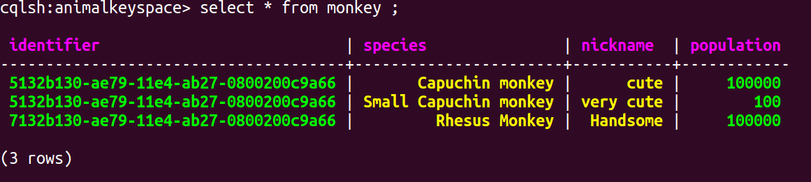
Now lets examine the data file. This will enable us to have a better understanding how data is actually stored on disk. To begin have a point of comparison lets first run a simple Select command:

Select * from monkey;

You should see output similar to the following screenshot. Please note the about query is for demonstration purposes and you will hardly ever run a query without at least part of primary key in your predicate.

No lets see what the underlying format looks like. The sstable2json is a utility can be used to converts a binary SSTable file into a JSON. This is a great tool to enable users to understand and visualize SSTables.

Lets convert data inserted into our Monkey table into JSON. In order to do so navigate to $ApacheCassandraInstallDir/bin directory and execute the following command.

./sstable2json $YourDataDirectory/data/animalkeyspace/monkey/animalkeyspace-monkey-jb-1-Data.db

On running the above command I get the following output.

[
  {
    "key": "5132b130ae7911e4ab270800200c9a66", // The row/partition key
    "columns": [                               // All Cassandra internal columns
      [
        "Capuchin monkey:",                    // The Cluster key. Note the cluster key does not have any data associated with it. The key and the data are same.
        "",
        1423586894518000                       // Time stamp which records when this internal column was created.
      ],
      [
        "Capuchin monkey:nickname",           // Header for the nickname internal column. Note the cluster key is always prefixed for every additional internal column.
        "cute",                               // Actual data
        1423586894518000
      ],
      [
        "Capuchin monkey:population",        // Header for the population internal column
        "100000",                            // Actual Data
        1423586894518000
      ]
    ]
  }
]

As mentioned in previous articles on should try and visualize a Cassandra column family as a map of sorted maps i.e. Map<rowkey, sortedmap<columnkey,="" columnvalue="">>). The data inserted into the Monkey table can is visualized as a map below.

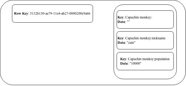
Note the partition key 5132b130ae7911e4ab270800200c9a66 is the row key and the key for our outer map. "Capuchin monkey:" is our cluster key and the first entry in the inner sorted map. The first entry of the sorted map does not have any data as the key and the data are the same.  Subsequent map entries create their key by suffexing the column name to the cluster key. "Capuchin monkey:nickname" key is a result of the cluster key + the column header nickname. The data part contains the actual data for the column.

The image below visually depicts the linkage between the CQL row the resulting SSTable and a logical map of sorted maps.

Now lets insert two more CQL rows. The first row inserted will have the same partition key but will change the cluster key. The second row inserted will have a new partition and cluster key.

 INSERT INTO monkey (identifier, species, nickname, population) VALUES ( 5132b130-ae79-11e4-ab27-0800200c9a66, 'Small Capuchin monkey', 'very cute', 100); INSERT INTO monkey (identifier, species, nickname, population) VALUES ( 7132b130-ae79-11e4-ab27-0800200c9a66, 'Rhesus Monkey', 'Handsome', 100000); 

Lets once again first run a simple select command:

Select * from monkey;

You should see output similar to the following screenshot:

Next navigate to

$ApacheCassandraInstallDir/bin

and execute

./nodetool flush animalkeyspace ## Second nodetool flush of the exercise
./nodetool compact animalkeyspace ## Never do this on a production system

Your data will be in a data file will no be in animalkeyspace-monkey-jb-3-Data.db. Note the unique node level table number is set to 3. This is because the second nodetool flush would have created a data file with the unique node level table number 2. The compact command would have combined data in file 1 and 2 and created a new file 3 with the aggregated data. More on compaction in later blog posts.

Lets convert the data in our newly created SSTable into JSON. Execute the following command extract the JSON representation of animalkeyspace-monkey-jb-3-Data.db:

./sstable2json $YourDataDirectory/data/animalkeyspace/monkey/animalkeyspace-monkey-jb-3-Data.db

On running the above command I get the following output:

[
  {
    "key": "5132b130ae7911e4ab270800200c9a66",
    "columns": [
      [
        "Capuchin monkey:",
        "",
        1424557973603000
      ],
      [
        "Capuchin monkey:nickname",
        "cute",
        1424557973603000
      ],
      [
        "Capuchin monkey:population",
        "100000",
        1424557973603000
      ],
      [
        "Small Capuchin monkey:",
        "",
        1424558013115000
      ],
      [
        "Small Capuchin monkey:nickname",
        "very cute",
        1424558013115000
      ],
      [
        "Small Capuchin monkey:population",
        "100",
        1424558013115000
      ]
    ]
  },
  {
    "key": "7132b130ae7911e4ab270800200c9a66",
    "columns": [
      [
        "Rhesus Monkey:",
        "",
        1424558014339000
      ],
      [
        "Rhesus Monkey:nickname",
        "Handsome",
        1424558014339000
      ],
      [
        "Rhesus Monkey:population",
        "100000",
        1424558014339000
      ]
    ]
  }
]

The above data can be visualized as depicted in the following image.

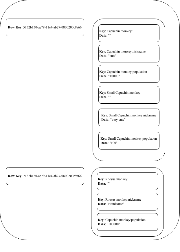
Note the second insert statement just appends to an existing row key with new cluster keys. Thus the three new columns with keys  Small Capuchin monkey:, Small Capuchin monkey:nickname and Small Capuchin monkey:population are added to the 5132b130ae7911e4ab270800200c9a66 row. The third insert statement created a whole new row with a pration/row key 7132b130ae7911e4ab270800200c9a66.

If you have reached this for far congratulation and I hope you now have a basic understanding of CQL and its effects on the underlying structures.