Understanding JVM Garbage Collection – Part 1

Java is a popular language for business and enterprise computing. Java and the JVM have enjoyed enormous success over the last two decades.

Java was initially considered a slow language (late 90's). That changed with the introduction of the HotSpot virtual machine in April 99. HotSpot improved performance via "just in time" compilation and adaptive optimisation. Since Apache Cassandra is written in Java, optimising Apache Cassandra requires a good understanding of the JVM's inner workings.

The JVM is a complex application and has five critical subsystems.

• The ClassLoader - Loads class files into the JVM.

• The Interpreter - Executes instructions loaded via the ClassLoader.

• JIT Compiler - Monitors the interpreter and produces optimised machine code for identified hot spots.

• Garbage Collector - The JVM decouples application logic from memory management by providing garbage collectors. Garbage collectors track memory allocated on the heap and reclaim's space occupied by unused objects.

• Runtime Data Area - This holds code and application data required to execute a program.

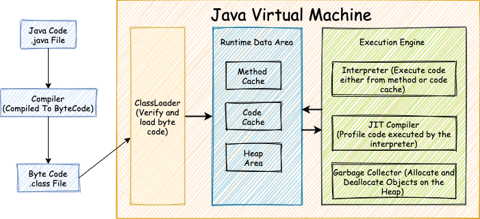
  JVM Overview

Java programs are stored in a .java file. These files are compiled into byte code using a Java compiler. Executing a Java program instructs the JVM to load all byte code associated with the program into memory via ClassLoader. The ClassLoader is responsible for loading, linking, and initialising all byte code associated with the program. The loaded classes are store in the method cache. The interpreter is responsible for compiling and executing the loaded code. The interpreter fetches instructions from the method cache. It is responsible for translating instructions in the method cache into assembly code. The generated assembly code executes on the target hardware.

To improve performance, the Just In Time (JIT) compiler continuously profiles compiled/executed code. The JIT compiler identifies frequently interpreted code, i.e., hot spots. Identified code hot spots are pre-compiled and placed in the code cache. For all future executions, the interpreter fetches the code from the code cache instead of the method cache.

The Garbage collector is responsible for allocating and deallocating dynamic memory to meet the application needs.

Due to the complex nature of the JVM, it is hard to reason about Java performance. Approach JVM performance as an experimental science.[^4]

The ClassLoader, Interpreter and the JIT Compiler are hardly ever the cause of performance problems. To tune Apache Cassandra, we need to optimise the Garbage Collector for our workload. It is the only subsystem that we can optimise. Optimising the Garbage Collector requires a deep understanding of garbage collection in the JVM.

Garbage Collection Basics

Overview

Applications have three types of memory allocations.

• Static Allocation - This type of memory is allocated at program startup and exists for the entire life of the program. Global, file scoped, and static variables come under the umbrella of statically allocated variables.
• Automatic - This type of memory is allocated upon entry into a block of code. It exists for the duration of that block. Automatic memory is essentially memory allocated on the stack.
• Dynamic Allocation - This is memory allocated by the program and exists until the program cleans it up. In Java, dynamic memory is allocated in a designated area of the application's memory called the heap. The heap is automatically cleaned using a Garbage Collector (GC).

Languages such as C, C++ and Objective-C make memory management the responsibility of the programmer. The programmer is responsible for allocating and deallocating memory. Unfortunately, experience has shown that this approach is error-prone, complicated and expensive.

Java solves this problem by using a Garbage Collector (GC). A GC performs the following operations:

• Allocates space/memory, as requested by the application, for newly created objects.
• The GC identifies live objects, i.e., memory currently used by the application.
• The GC reclaim space occupied by dead objects, i.e., is responsible for freeing unused memory for reuse.

In Java, the GC allocates and deallocates memory on the heap. The GC keeps track of all objects allocated on the heap and automatically removes unused/dead objects. A GC is not free and comes at a cost, i.e. application pauses aka stop the world pauses. Most GC algorithms need to pause all application threads while unused objects are purged from the heap. Using a GC means that the programmer abdicates control on when memory is allocated or deallocated.

The GC is a complex piece of code that is tightly woven into the JVM. Garbage collectors have a number of responsibilities that include but not limited to:

• Determines the initial memory layout of the heap. If required, re-layouts the heap to optimise the program.
• Determines the layout of objects and their size
• Tracks objects over their lifetime
• Injects Just In Time (JIT) compilation codes

Your choice of GC has a significant impact on the performance of your application. A GC is chosen for a lifetime of a program and cannot be switched at runtime. GC is a complex topic that must be understood to tune any Java application. The JVM has numerous GC implementations with different tradeoffs. It is the implementer's responsibility to choose the correct garbage collector for their workload. Tuning the GC necessitates understanding your workload, performance requirements and the pros and cons of the GC algorithm used.

GC Approaches

At a high level there are two main approaches to GC:

Reference Counting

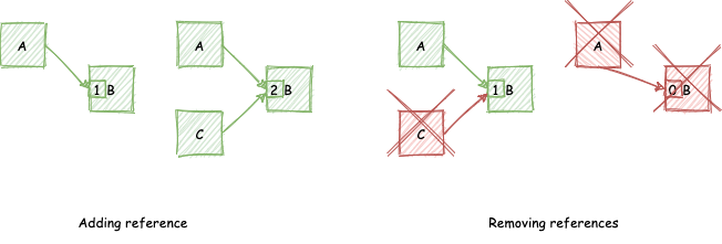
Reference counting keeps a count of the number of references to an object. Object creation or referencing results in bumping up the reference count. Object dereferencing results in reducing the reference count. When the reference count reaches zero, the object is deallocated. Due to its simplicity, reference counting is used in several languages such as Python, Awk, and Perl. Reference counting's main advantages are:

• Memory is reclaimed as soon as the object is no longer referenced by any object. Memory can be reclaimed as an object becomes garbage.
• Allocation/Deallocation costs are distributed throughout the computation.

The main disadvantages of reference counting are:

• All read and write operation comes with a reference counting overhead.
• Reference count manipulations must be atomic to prevent race conditions between objects mutating the reference count.
• Reference counting cannot reclaim cyclic data structures.

Reference Counting

The image above illustrates the reference counting process with respect to object B. B's reference count is bumped up as new objects refer to B. Similarly B's reference count is bumped down as objects no longer refer to the object. Once the objects reference count is zero, the object is deallocated.

Another good way to understanding reference counting is via the Python REPL.

Python uses reference counting as one of its GC strategies. It also has a system library that enables one to access the objects current reference count. Note the sys.getrefcount will return the reference count plus one as it is also referring to the object when invoked. Observe how the reference count to objects increments when a new object refers to it. Similarly, the reference count decrements when an object reference is removed.

Tracing Garbage Collection

As opposed to reference counting tracing garbage collectors do not free memory immediately. GC is triggered when the system is running low on memory. The GC traces reachable objects starting from root objects also known as GC roots. A GC root is a pointer into a memory pool from outside that memory pool, i.e. an object that is accessible from outside the heap. In Java GC roots include, but not limited to,

• Pointers from local variables allocated on a stack.
• Pointers form the active Java thread.
• Pointers from Java native code handlers.
• Pointers from classes loaded into the system class loader.

The algorithm traces the entire object graph starting from the root nodes. Objects are marked as they are encountered. Marking is done by setting a flag on the objects or using some external data structure. After tracing is finished, all unreachable objects are known and eligible for completion. All objects that are not part of the object graph that originates from a GC root are eligible to be reclaimed to free unused memory.

A popular tracing algorithm is the Mark and Sweep algorithm.[^2]

The image above illustrates tracing GC at a high level. The application is paused when GC is required. The object graph from the GC root is traced. Dead objects (F) is identified and removed. The application is unpaused and continues its normal processing.

As we will discover, there are various approaches and strategies used when implementing a tracing garbage collector. At a high level, tracing garbage collectors are evaluated using the following three parameters:

• GC throughput - The amount of time the CPU spent performing GC.
• GC latency - The amount of time taken to perform individual garbage collection.
• GC footprint - The amount of memory used to execute the application.